GIS analysis in Jupyter Notebook

Introduction

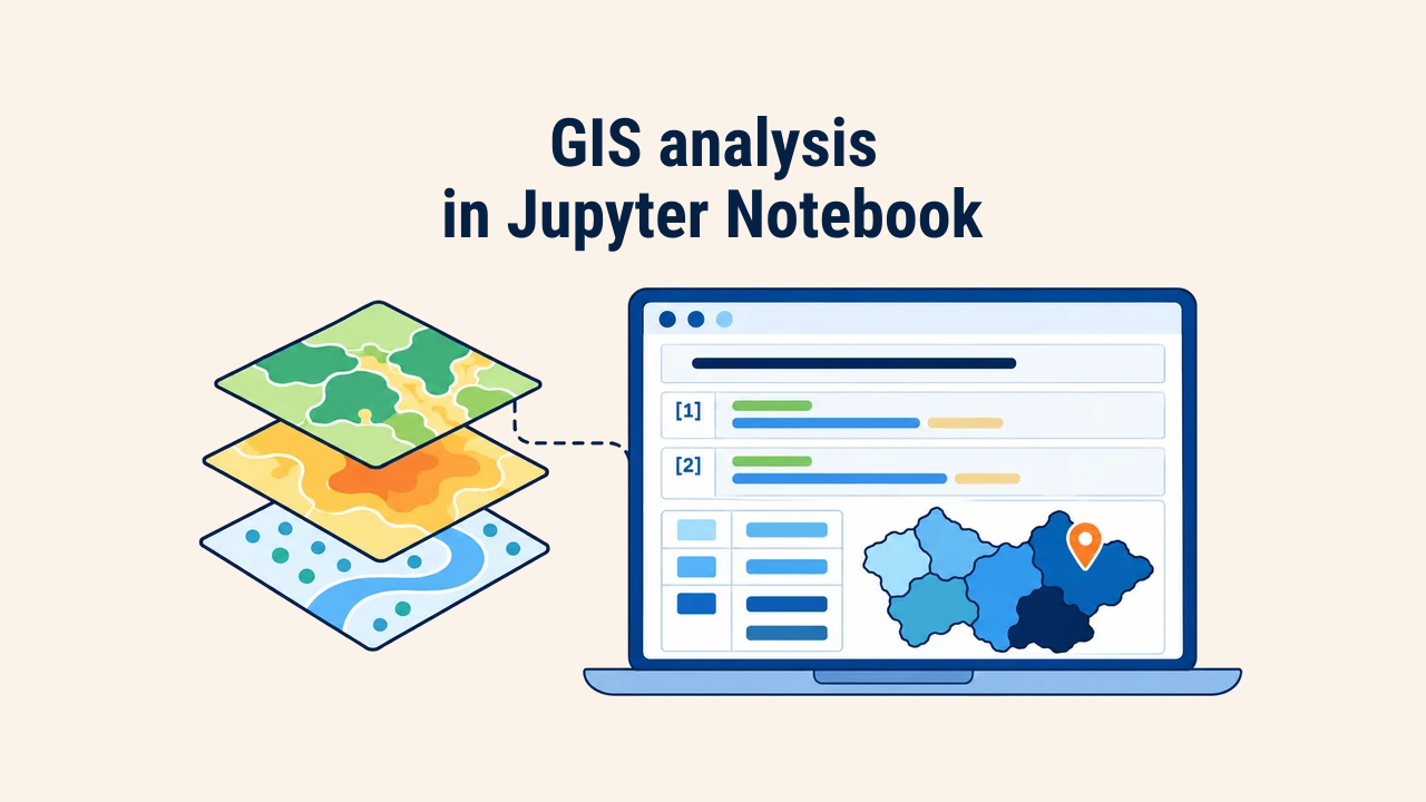
A Jupyter Notebook is an interactive computing environment that integrates executable code, computational outputs, and narrative documentation within a single unified web document. Code is structured into modular blocks termed cells. Each cell executes independently, rendering dataframes, statistics, or vector map displays directly beneath it.

In GIS workflows, this setup is highly advantageous: analysts load layers, verify coordinate systems and attributes, inspect map outputs interactively, and determine subsequent processing steps based on intermediate findings. At the same time, notebooks introduce subtle operational risks that compromise reproducibility if ignored.

Notebook structure

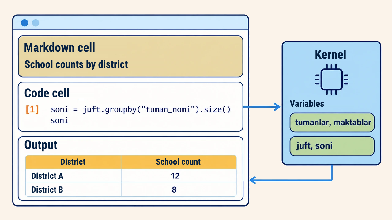
Notebook files use the .ipynb extension and contain two primary cell types. Code cells store and execute Python statements while displaying runtime results. Markdown cells hold formatted documentation, LaTeX formulas, tables, and hyperlinks explaining the methodological reasoning behind analytical steps.

Execution is managed by a background Python process known as the kernel. The kernel maintains variables and data structures in memory across executions, meaning layers imported in an early cell remain accessible throughout subsequent cells. Modern teams generally run notebooks within multi-panel JupyterLab interfaces or IDEs like VS Code.

Diagram showing the connection between Markdown cells, code cells, output cells, and the background execution kernel in Jupyter Notebook

Building analysis cell by cell

Consider a representative workflow: loading Tashkent district boundaries and school points to calculate school density across municipal jurisdictions. The first cell loads and audits the input layers:

import geopandas as gpd

tumanlar = gpd.read_file("toshkent.gpkg", layer="tumanlar")
maktablar = gpd.read_file("toshkent.gpkg", layer="maktablar")
print(tumanlar.crs, maktablar.crs, len(maktablar))

This immediately confirms matching CRS definitions and expected record counts. The subsequent cell executes the spatial join and aggregation:

juft = gpd.sjoin(maktablar, tumanlar, predicate="within")
soni = juft.groupby("tuman_nomi").size()
tumanlar = tumanlar.merge(soni.rename("maktab_soni"),
                          left_on="tuman_nomi", right_index=True, how="left")
tumanlar["maktab_soni"] = tumanlar["maktab_soni"].fillna(0)

The final assignment fills zero values for districts without schools. Inspecting intermediate results cell-by-cell isolates bugs immediately, allowing targeted adjustments without executing the entire script from scratch.

Interleaving brief Markdown notes between code blocks—documenting data vintages, coordinate references, and boundary edge cases—ensures collaborators can trace the analytical narrative effortlessly.

Interactive mapping

The explore() method in GeoPandas renders an interactive, pan-and-zoom web map directly within the notebook cell output. Built on folium and Leaflet, it requires the folium dependency:

tumanlar.explore(column="maktab_soni", cmap="Blues", legend=True)

Clicking a feature opens an interactive tooltip displaying underlying attributes. This capability quickly reveals coordinate reference offsets, attribute omissions, or polygon slivers. When static publication figures are needed, standard plot() calls suffice.

Interactive maps inject GeoJSON geometries directly into the browser DOM. Rendering tens of thousands of complex vertices slows notebook responsiveness and inflates document file sizes. For massive vector layers, filter subsets or simplify geometries before launching interactive maps, or fall back to static raster plots.

Execution order risks

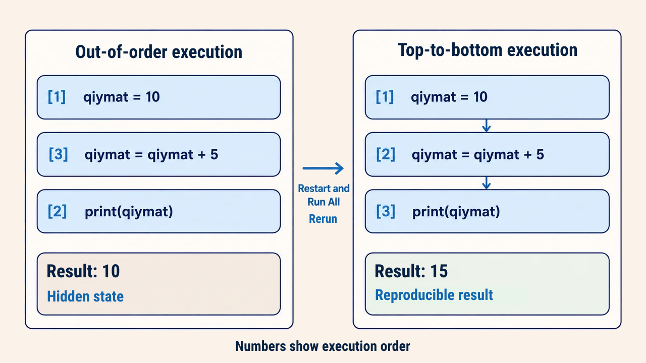
The principal vulnerability of computational notebooks is hidden state. Cells can be executed in arbitrary non-linear order, yet the kernel remembers all past memory states. If a transformation cell is executed multiple times or references variables from a deleted cell, displayed code diverges from actual memory states.

Execution counter badges such as [3] beside cells reflect actual execution sequences. Disordered badge numbers indicate unverified results. After completing an analysis, always execute a clean end-to-end run (Restart and Run All). Consistent outputs confirm that the notebook is truly reproducible.

Comparison diagram illustrating hidden state when running cells out of order (1, 3, 2) versus clean execution with Restart and Run All

From notebook to script

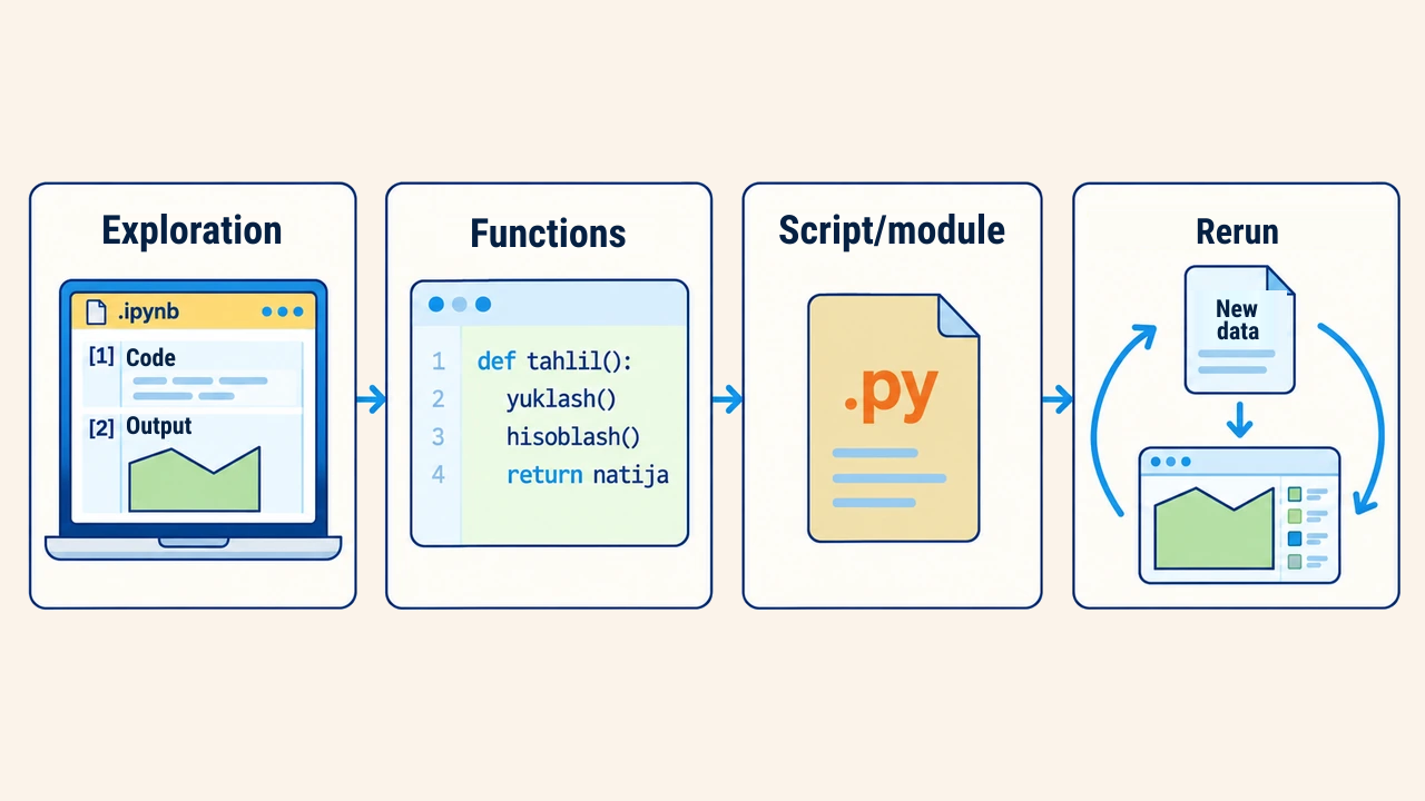
Jupyter Notebooks excel at exploratory data analysis, proof-of-concept modeling, and documentation. However, when recurring monthly updates run in production or integrate into automated pipelines, refactor code into standalone .py scripts. Standard practice involves packaging validated notebook logic into parameterized functions, leaving the notebook as a lightweight orchestration runner.

Version control also requires attention. Because .ipynb files store rich outputs and base64 images inside JSON arrays, Git diffs quickly become cluttered. Clearing cell outputs before committing or using text-based notebook converters keeps code repositories clean and auditable.

Workflow diagram showing notebook exploration, code refactoring into functions, script export, and automated execution on new data

Conclusion

Jupyter Notebook structures GIS analysis into modular, auditable steps, providing immediate feedback through data tables and interactive web maps. Markdown cells ensure analytical reasoning is preserved alongside execution code.

Trustworthy results demand that notebooks replicate identically when executed top-to-bottom in a fresh kernel, with production workflows transitioned cleanly into modular Python scripts.